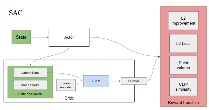
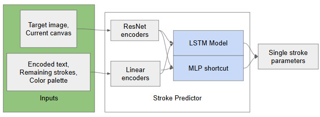
The Actor structure is on the left and the SAC training structure is on the right.
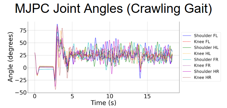
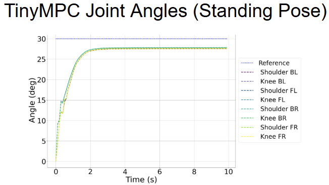
Stable gaits were able to be optimized using MJPC. These gaits were then successfully adapted to TinyMPC in Mujoco. The graphs show a walking gait from MJPC and a standing trajectory from TinyMPC, respectively.
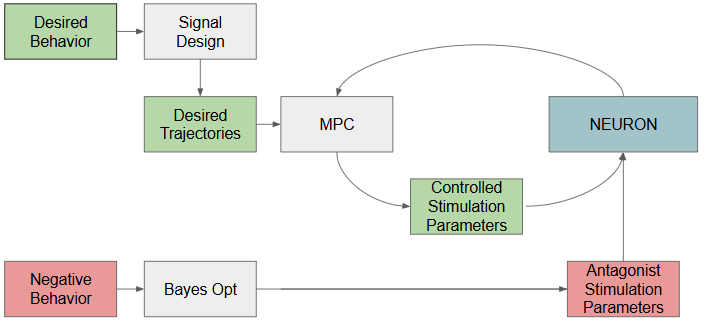
The antagonistic behavior was simulated by using Bayes Optimization to find the parameters that produced the unwanted behavior in the neurons. MPC was then run to correct for this behavior.
While the results we got from this project were not what we had hoped for, we believe there is potential in using this with some future work:
1. Model multi-neuron interactions
Better capture PV and Pyr coupling dynamics.
Modeling interactions between the types of neurons could reveal cruical control information
2. Upgrade simulator state representation
Having a simulator that can output continuous soma voltage would allow for finer control.
TDMPC:
TDMPC leverages a distribution over trajectories to perform model predictive control, enabling robust decision-making under uncertainty by optimizing over likely future outcomes. It combines planning and control using learned or analytic dynamics.
Dreamer:
Dreamer is a model-based reinforcement learning algorithm that learns a latent dynamics model and uses it to imagine future trajectories, optimizing policies entirely in the latent space for sample-efficient learning.
DDQN:
DDQN improves upon the standard DQN by decoupling action selection and evaluation, reducing overestimation bias and enabling more stable value-based learning in discrete action spaces.
General Advantage Estimation (GAE):
"The [data set] is related to a smart home environment where sensors retrieve information about temperature, light, humidity, CO-Gas, motion, smoke, door and fan with different time interval since the behaviour of each sensor is different with the others."
This dataset was chosen for its applications to the real world, where information from various sensors or inputs will need to be interpreted to gleam some insight not readily available to the human eye.
Data preprocessing was done using a custom tranformer pipeline using pyspark that consisted of several stages in the following order:
Five different ML models were selected and tested on the vectorized data: a Logistic Regression (LR) model, a Random Forest (RF) Decision Tree model, both a shallow and a deep Neural Network (NN), and an autogenerated model created using Edge Impulse. Both the Logistic Regression and Random Forest models underwent hyperparameter tuning, where the regularization parameter and max iterations were tuned for the LR model and the maximum tree depth and number of trees were tuned for the RF model. The neural networks were tuned and ended up with the deep one consisting of 4 layers of 128 neurons, with a learning rate of 0.005 decaying at a rate of 0.995 and 20 epochs. The shallow NN consisted of two layers of 8 neurons with a learning rate of 0.05 without decay for 10 epochs. Finally, Edge Impulse AI was used to upload the data and create one final model to compare to.
| Algorithm | Testing Data Accuracy | Rank |
|---|---|---|
| Linear Regression | 83.11% | 5 |
| Random Forest Decision Tree | 86.76% | 2 |
| Deep Nueral Network | 83.21% | 4 |
| Shallow Neural Network | 83.31% | 3 |
| Edge Impulse | 95.2% | 1 |
| Metric | Required | Result |
| Lap Time | 400 s | 94.3 s |
| Max Distance off Track | 10.0 m | 7.38 m |
| Average Distance off Track | 5.0 m | 0.73 m |
| Metric | Required | Result |
| Lap Time | 350 s | 90.5 s |
| Max Distance off Track | 9.0 m | 8.93 m |
| Average Distance off Track | 4.5 m | 3.48 m |
| Metric | Required | Result |
| Lap Time | 250 s | 85.4 s |
| Max Distance off Track | 7.0 m | 6.79 m |
| Average Distance off Track | 3.5 m | 0.84 m |
| Metric | Required | Result |
| Lap Time | 250 s | 85.9 s |
| Max Distance off Track | 7.0 m | 6.77 m |
| Average Distance off Track | 3.5 m | 0.82 m |
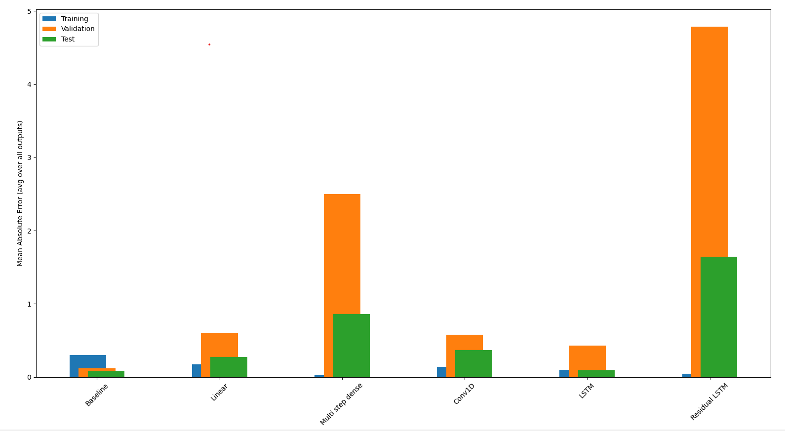
1D Conv
Multi-Step Dense
RMSE
Residual LSTM
LSTM
Linear
Baseline
This site was created with the Nicepage